Creating Consistent Spatial Calculations with Uber’s H3 Hexagons
Getting demographic data for a city or zip code is pretty straightforward — several APIs and data downloads exist to do so. But, for many reasons, these geographies have limitations (to name a few, zip codes are a function of USPS deliveries and city boundaries were established up to centuries ago — not exactly designed for data analysis).
I’ve tested out a couple different ways to overcome the arbitrary nature of these boundaries — everything from creating uniform boxes to developing drive (or walk) time polygons, depending on the use case.
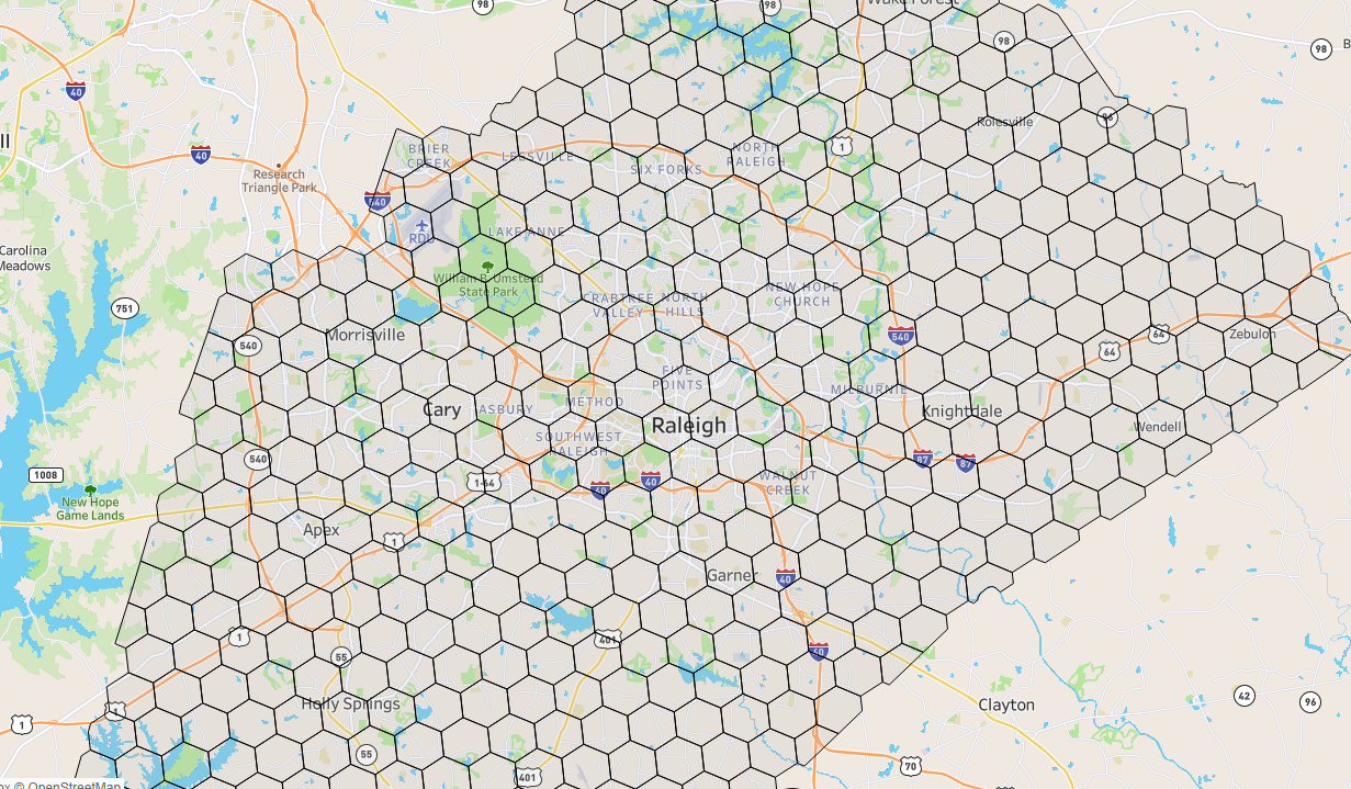
I recently became aware of the benefits of H3, a set of global hexagons introduced by Uber in 2018. The main idea is that a hexagon is the most beneficial shape for spatial analysis and can be used to create consistent calculations.
Each hexagon has a series of smaller hexagons that sit (mostly) inside of another, which creates a hierarchy that can be used for consistent referencing and analysis, all the way down to lengths of 2 feet for the edges.
This approach works well for point data — Where was a rider picked up? Dropped off? Any address or point of interest that has a latitude and longitude can be mapped into a hexagon.
What happens if we want to leverage the benefits of hexagon analysis but with demographic data? I found a lot of information on working with hexagons, but not bringing in demographic data, so I set out to combine the two.
When working with Census data, the most detailed view available with robust data reporting are Census Block Groups (read more on block groups here). Block groups are boundaries that typically have between 600 and 3,000 people, which makes them homogenous to study and use (areas this small tend to have similar people living in them).
However, because they’re population bound, there’s a lack of consistency to the size. For example, look at the census block groups in downtown Raleigh, NC below — some are smaller, some are bigger based on the distribution of the population.
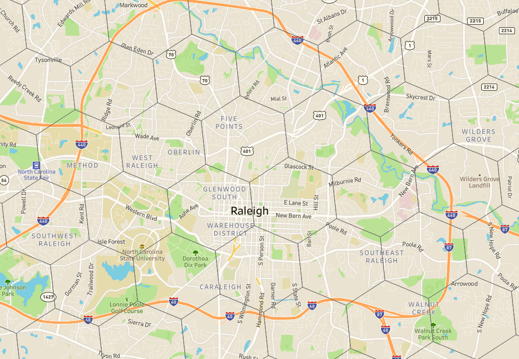
Contrast that to the hexagons (I’ve chosen a size at random for efficient analysis, but we could choose smaller or larger depending on the need), which are uniform in size with consistent borders.
Census block groups in downtown Raleigh, NC
Uber’s H3 Hexagons in downtown Raleigh, NC
So, the question becomes, how do we map the demographic information available in the census block groups to the uniform structure of the hexagons? How can we benefit from both the granularity of the census block groups and the uniformity of the hexagons?
The Big Picture — How can we solve this?
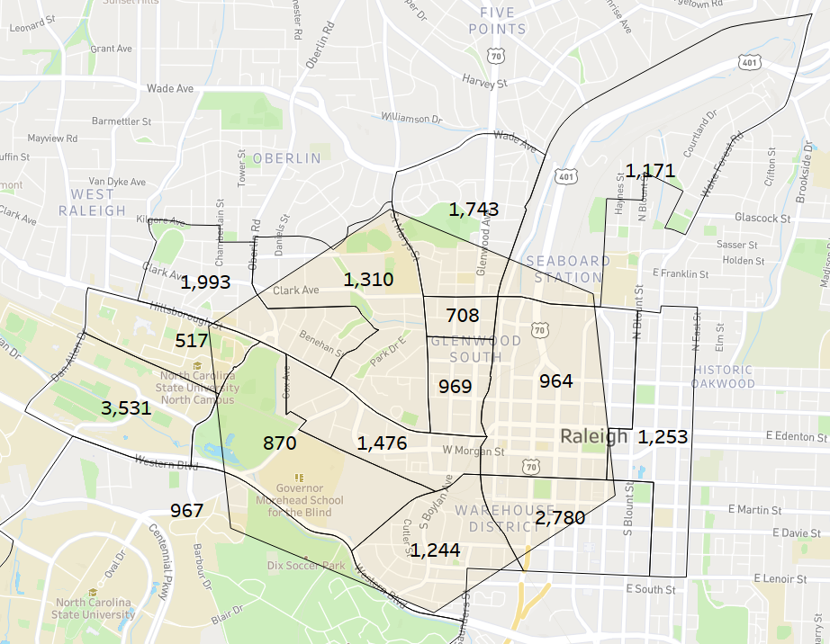
Let’s say we wanted to find the population within each hexagon — to be more specific, let’s look at a single hexagon. We can overlay the hexagon boundaries with the corresponding block group boundaries, bringing together something like the below…
Block group populations overlayed on an intersecting hexagon
Block groups that sit entirely within a hexagon are easy — we consider the whole population to be allocated to the hexagon (populations of 708, 969, and 1,476 in the middle of the hexagon). However, given the mismatch in shape, many have partial overlap, and this will only be more common with smaller hexagon sizes.
For any block group that intersects the hexagon, we can calculate the area overlap between the two shapes and proportionally allocate the population based on this calculation. If half of the block group overlaps, we consider half the population to be within the hexagon.
This assumption isn’t perfect — a population isn’t uniformly distributed within a block group — but for practical purposes, it gives us a “good enough” approach to be able to combine the two geographic shapes.
The Implementation
I’m going to demonstrate with code from the R programming language, but the approach is conceptually the same in Python or other languages.
We need two primary pieces of information to conduct the analysis — the block group shapes with their corresponding demographic data, and the hexagon shapes.
In R, we can leverage the tidycensus package to get data from the US Census API (you’ll need a free developer key). The get_acs function is the simplest way to acquire block group data, with a representative syntax below:
get_acs(geography = 'block group', year = 2020, variables = c(total_population = 'B01001_001'), state=37, county=183, output='wide')
The optional arguments define that we want block groups for the output, data from the 2020 5-year ACS, the total population variable identifier, the state of NC (FIPS 37), Wake County (code 183), and a wide output format.
Output from the get_acs function
From there, we need to match this to a shape (boundaries) for each block group. We can use the block_groups function from the tigris package and provide the state and county identifiers, which returns a shape file with the geometry polygons.
Example syntax to get a shape file for each block group in Wake County, NC
A simple join by GEOID can bring together the shapefile with the demographic information to create a single block group file. The output is then converted back to a shapefile using the sf package (more on that later) and transformed to the coordinate reference 4326.
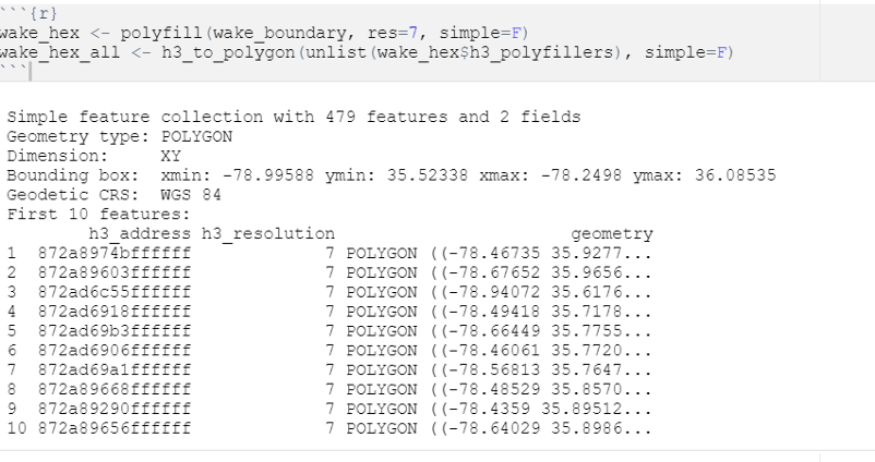
To get all hexagons in Wake County, I sourced the shapefile for Wake County (also using the tigris package, but the counties function) and then leveraged the h3jsr package to access the H3 hexagons.
The polyfill function finds all hexagons within a provided boundary (here, Wake County, home to Raleigh), and the h3_to_polygon function gives the shapes for each hexagon. The res = 7 argument defines what level of granularity we want for our hexagons (15 is the most precise, 0 is the largest).
The output is a series of hexagon reference IDs and polygon shapes.
Now, for each hexagon, we want to:
Find any block group that intersects (overlaps) with the boundaries of the hexagon
Find the percent overlap for the block group
Allocate the population in the block group according to the percent overlap
The sf package in R is a go-to package for spatial analysis. The st_intersection function looks for overlapping area of two shapes, and the following mutate function calculates the percent overlap. The output of this code will be all block groups that overlap, along with their area overlap.
Example output of the st_intersection function with additional data manipulation
The final step is to convert the population to a numeric, multiply the population by the percent intersect to get an adjusted population, and sum the adjusted population for a total in the hexagon.
For example, in the above image, a population of 2,911 with ~11% overlap becomes an adjusted population of ~317.
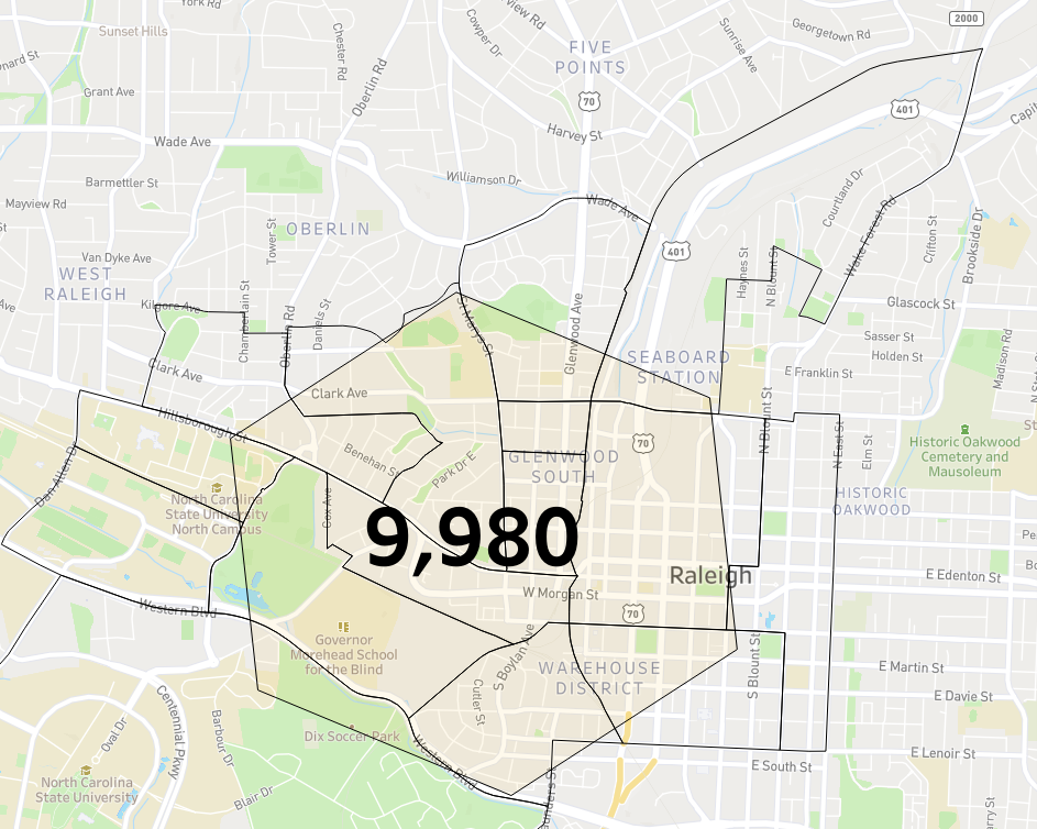
Returning to our earlier example, this approach gives an estimated hexagon population of 9,980. Looking again at the populations within each of the block groups, a visual comparison suggests this probably isn’t too far off.
Estimated hexagon population
Overlapping census block group populations
This approach has limitations when the hexagon / block groups have large overlap with protected land, like parks or bodies of water, which will be most impactful for small hexagons in more rural areas. Given the population density of most cities and immediate suburbs, I’d expect this approach would be directionally helpful in the majority of cases.
Extending the Analysis
Population was just used as an example, but anything reported at the block group level could be used. What’s the median household income for a hexagon? How many households are there? What percent of households have children? Adding to the variables collected in the get_acs function enables other options for how to analyze and aggregate the data.
This can also be combined with any point of interest data that can be aggregated into the hexagons, for example by finding areas with a high density of a given point of interest, then describing that hexagon’s demographic composition.
While not perfect, this provides an approach to create consistent calculations for spatial analysis and trends. In the aggregate, we’d expect the data to be directionally useful — if we calculate that one hexagon has 20% higher population than another, we’d be reasonably certain that the first hexagon has higher population, even if not exactly 20%.


